Monday 16 July 2012

Living with Linux Desktops: KDE4 V Xfce on Opensuse 12.1

Here is a brief comparison of Xfce desktop and KDE desktop that comes with opensuse linux 12.1. The screen shots for the konsole using top command for memory and system monitor shows the difference. Notable is that KDE Dolphin uses 25MB whereas, Thunar the default file browser for Xfce used 17MB. Half of Dolphin. On CPU and memory Xfce desktop has half resource usage compared to KDE4. I have not used KDE plasma graphics too much on my desktop. KDE4 desktop is configured to use clean looks and use suse look and feel. Having Xfce on an older hardware can make it faster or comparable to a new hardware running latest operating system. 

File Manager
----------------
Dolphin 25MB
Thunar 17MB

Comparison
----------------
          CPU(2cores)      Memory
KDE      6, 3.9%                      0.30 GB / 2.0 GB
Xfce     2, 3.9%                      0.16GB / 2.0 GB

Xfce feels responsive and faster. In fact too fast. The one disadvantage of Xfce is that, sometimes the widgets/panel apps don't work. For example, the window manager had to be started manually at command line. Or the windows did not have close/minimize/maximize buttons. Again, Lock Screen does not seem to invoke any response from Xfce and also resuming after hibernating does not prompt for password by default.

Screens

KDE Top and System Monitor

Xfce Top and System Monitor

Monday 9 July 2012

Friend Suggestion like Facebook, Google+ or Product Suggestion like Amazon: Implementing for your own web app, site

This is an application of Apache Hadoop MapReduce framework. Facebook has a feature that says that, some people may be your friends. This is calculated based on a number of factors such as common friends, likes, visits to profile,
comments made etc. Basically the interactions is logged, analyzed and put through a kind of weighted matrix analysis and the connections which are above a threshold value are chosen to be shown to the user.

Problem: An input file of 1GB size with the logs of interactions among 26,849 people. To keep the data manageable on my computer, I am creating random logs with interaction of 1000 people with the rest of the people on the, say social
networking site. Gathering and presenting this data to map reduce is itself a job. In our case, these 1000 people need friend suggestions.

Solution: Here this is done in a Single map reduce job although, more data and intermediate jobs can be added in real life. The mapper for the job takes each interaction and emits the user pair and interaction statistics. For example,
Sam Worthington has 1 profile view, 2 friends in common, 3 likes with Stuart Little. so the out put of the mapper here is . We could use the userid across the site rather than a name. For each person interacting with Stuart Little a record like this is produced.

The reducer simply takes the output of the mapper and calculates the sum of the interactions per user-user pair. So, for a week of interactions the record from the reducer may be, for example, . This is got by summing up the interactions by the reducer. Then, each interaction can be given a weight/value then, the number in the record can be multiplied by the weight and summed. Any calculation is ok as long as it give a meaning result based on the interaction types. Then, interactions with a score larger than a threshold can be chosen to be presented to the user when they login.

Other factors like user interests, activities etc can also be accounted for. Here we can simple treat each as a user and emit a record if there is a related activity in user's profile and proceed as usual. The same approach can be applied to ad serving utilizing info from user profile and activity. A Combiner and mutiple jobs can be used to get more details too.

Results: For 1GB, in real life big data approaches > 2TB, of randomly generated log of interactions of 26K+ people with a select 1000, the mapreduce program gave the friend suggestions in 13 mintues on my laptop with a pseudo distributed Hadoop configuration. So, if you have a few tera bytes of data and 10 computers in a cluster you can get the result in say 1.5 hours. Then all that is needed would be to consume the friend suggestions via a regular db / webservice and present it to the user when they log in.

Screen shots of the Map Reduce job run on pseudo distributed Hadoop:

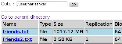
1) Copying the data to Hadoop Distributed File System


2) Running the jobs

3) Status on Hadoop admin interface.

4) Friend Suggestions with statistics.


5) Job code

6) Mapper

7) Reducer

Sunday 1 July 2012

Apache Hadoop Map Reduce - 1

Hadoop is a map reduce framework that allows for parallel distributed computing. The criteria for adopting Hadoop is that, the same operations are performed on records and records are not modified once created. So Reads are more frequent than write in a traditional relational database system. The advantage of Hadoop or a Map Reduce frame work comes into action when the data is large enough ~ 1TB. Above this point data is referred to as big data approaching PetaB. At such a point it is better to throw multiple machines at the task rather than to use a single machine with parallel programming. The technique used is Map Reduce which deals with Key and value pairs.

A map operation is performed on records whose inputs and outputs are key value pairs themselves. The output is merged, sorted and submitted to a reduce operation which combines and generates the output. For example, we have 12 years of student records for examinations across 15 subjects. The total number of records is 5,700,000. On this data set we can find operations such as highest score on a subject over the years, total failure reported across the year etc. To find the total failures, the map operation outputs a key value pair   every time it encounters a failed exam. The reduce job takes all such key value pairs and emits a Key value pair .

The hadoop standalone configuration on these records finished in ~ 35-40 seconds. The hadoop run start is shown here
 The run end is here
Output is here. 

The same on a pseudo clustered mode gives results for similar operations in ~40 seconds. The difference is that, the input files have to copied into the Hadoop distributed file system and the output needs to be copied/read from the HDFS. As shown here